CAM age, MAM age, FMM age…. Can I just have an age please?
/A luminescence age from a sample is typically calculated from a distribution of ages measured from multiple individual grains or multi-grain aliquots from that sample. The age (or De) distribution of samples where all of the grains have been sufficiently exposed to sunlight to deplete their signal prior to final deposition will be tightly clustered around a single value (assuming minimal or no grain-to-grain variations in environmental dose rate). Those samples where many grains contain a residual, unbleached signal, on the other hand, will exhibit a much more broad, or skewed age distribution. In this latter case, a calculated mean or average age will over-estimate the true age (or time of final deposition) of the deposit.
The Central Age Model (or CAM) is a statistical model typically used to calculate the age from De distributions in samples that have been well-bleached prior to deposition. If this model is applied to samples of several hundred years in age or older, it is typically applied to log-transformed De values to take into account the fact that the De standard errors typically increase with the size of the De estimates. When it is applied to very young, or modern samples, where no strong correlation between De values and their standard errors exist however, it is typically applied to unlogged data.
The CAM yields two parameters:
1) the central dose (δ), which is essentially the geometric mean of the De distribution, and
2) and the overdispersion (σ), or the relative standard deviation of this distribution.
The overdispersion parameter represents the “spread” in the De distribution that remains after all measurement errors specific to each grain/aliquot (also known as the “within-aliquot variation”) have been taken into account. When σ is non-zero or high, we may infer that: i) some grains have been insufficiently bleached prior to deposition, ii) there has been mixing between sedimentary layers of different ages, and/or iii) there are grain-to-grain variations in environmental dose rate not taken into account in our dose rate estimate.

A multi-grain aliquot De distribution from a partially bleached sample collected below an intertidal indigenous clam garden wall on Quadra Island, BC, Canada (Neudorf et al., 2017). Grey shading in the radial plot marks ±2σ of the CAM De value (~5 ka), and the solid line marks the younger MAM De value (~4 ka). Click here for an explanation on how to read a radial plot.
The Minimum Age Model (or MAM) is typically applied to samples that are known to have received insufficient light exposure to re-set the luminescence signals in all grains prior to final deposition. This often occurs in colluvial or waterlain deposits. This model assumes that the true (log-transformed) De values are drawn from a truncated normal distribution, where the lower truncation point (γ) corresponds to the average true log De of the population of fully bleached grains.
The MAM yields four parameters:
1) the minimum dose (γ), which corresponds to the minimum age of the deposit,
2) the proportion (p) of grains/aliquots in the De distribution that comprise the minimum age,
3) the mean (µ) and standard deviation (σ) of the truncated normal distribution from which the log-transformed De values are assumed to be derived.
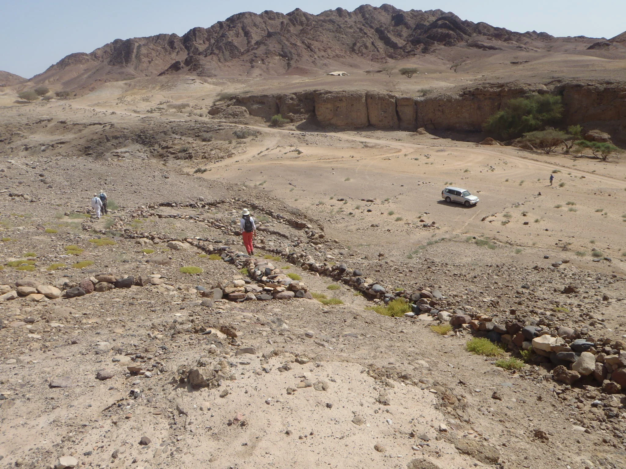
The Finite Mixture Model (or FMM) is applied to samples with mixtures of grains derived from two or more sedimentary units of different ages. Sediment mixing can occur during soil forming processes, bioturbation, infilteration of finer grained material into coarser grained deposits, or human activities such as trampling, ploughing or digging. In these situations, the FMM is used to distinguish between individual De components in the distribution, the absolute number of which, is not always known a priori.
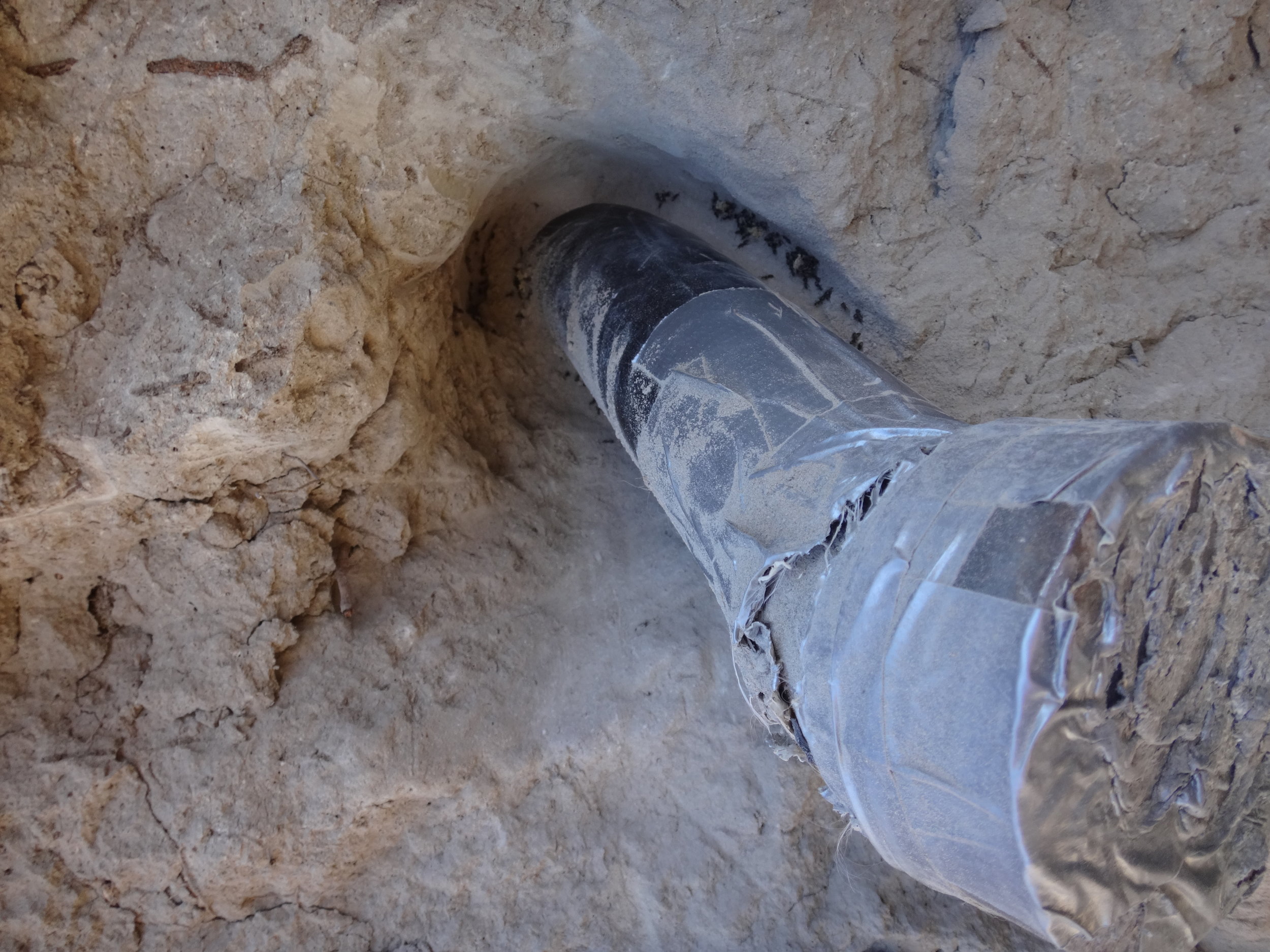
This OSL sample tube has intersected an ant burrow. Sediment mixing can occur when roots or insects burrow into the substrate, bringing recently sun-bleached grains from the surface down into older sedimentary units. Photo credit: Christina Neudorf
Application of the FMM to a De distrbution is an iterative process that determines:
1) the number (k) of discrete De components in a distribution,
2) the relative proportions of grains (π) in each component,
3) and the mean (µ) and standard deviation (σ) of each component.
It is generally not advised to apply the FMM to multi-grain aliquot De distributions, as multi-grain aliquots may contain grains from more than one De component. If the FMM is applied to multi-grain aliquot data, it may generate pseudo- or “phantom” De components with doses that fall between those of the true De components.

A single-grain (black dots) and multi-grain aliquot (white triangles) K-feldspar age distribution from a sample collected from alluvial sands in the Middle Son Valley, Andhra Pradesh, India (Neudorf et al.2014). The solid lines plot the ages of three FMM age components detected in the single-grain data that are interpreted to represent a mixture of older cutbank deposits and younger fluvial sands. The youngest (third) component is interpreted to represent bioturbation as roots penetrating overlying soils translocate grains from the surface down to the sample site. The shaded region marks ±2σ of the MAM De value calculated from the multi-grain aliquot data. Click here for an explanation on how to read a radial plot.